Seq2Seq from Scratch: Building an English-to-French Translator with LSTMs

A complete guide to understanding and implementing Sequence-to-Sequence models.

---

Table of Contents

1. What is Seq2Seq?
2. The Architecture
3. Vocabulary: Converting Words to Numbers
4. The Encoder
5. The Decoder
6. Hidden State & Cell State Explained
7. Training: Teacher Forcing
8. Inference: Greedy Decoding & Beam Search
9. The Bottleneck Problem
10. How to Actually Remember This

---

What is Seq2Seq?

Seq2Seq (Sequence-to-Sequence) is an architecture designed for tasks where both input and output are sequences of variable length. Perfect for:

• Machine Translation (English → French)
• Text Summarization (long article → short summary)
• Chatbots (question → answer)

The key challenge: input and output can have different lengths.

Input:  "how are you"     (3 words)
Output: "comment allez vous" (3 words) ✓ same length

Input:  "hello"           (1 word)
Output: "bonjour"         (1 word) ✓ same length

Input:  "thank you"       (2 words)
Output: "merci"           (1 word) ✗ different length!

Traditional neural networks need fixed input/output sizes. Seq2Seq solves this elegantly.

---

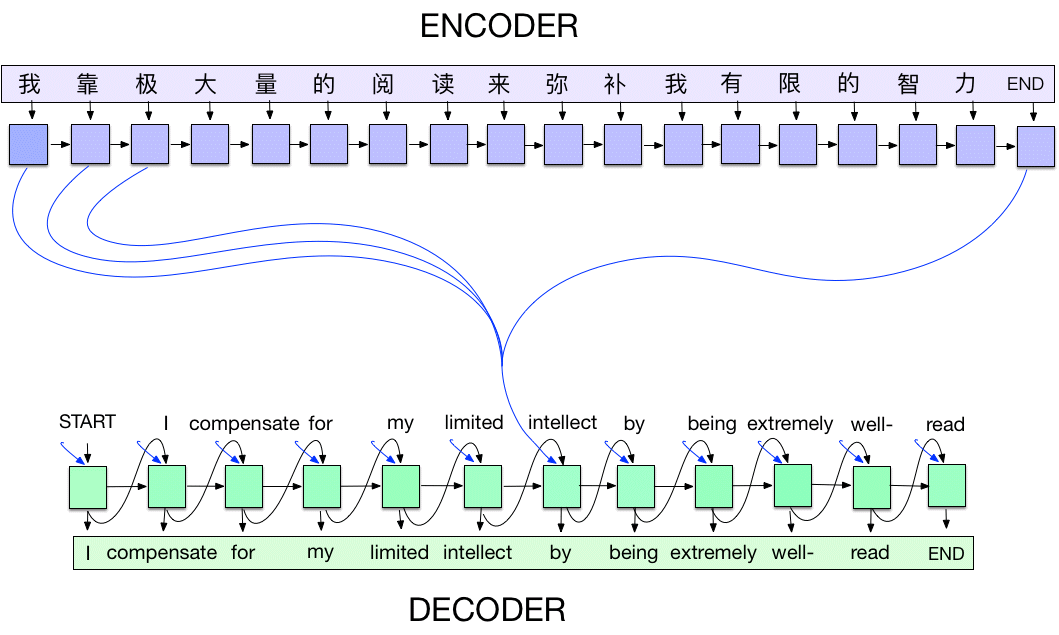
The Architecture

Seq2Seq has two main components:

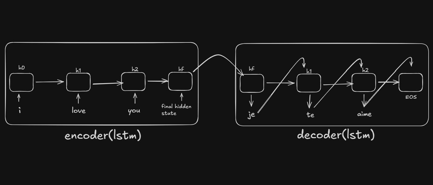
English: "i love you"  →  [ENCODER]  →  Context Vector  →  [DECODER]  →  "je t aime"

Encoder

• Reads the input sentence word by word
• Compresses the entire sentence into a fixed-size context vector (the final hidden state)
• This vector captures the "meaning" of the input sentence

Decoder

• Takes the context vector as its initial state
• Generates the output sentence word by word
• At each step, predicts the next word based on previous words + context

Why LSTM?

• LSTMs can remember long-range dependencies (e.g., subject-verb agreement across many words)
• They solve the "vanishing gradient" problem of vanilla RNNs
• They have a "cell state" that acts as a highway for information

---

Vocabulary: Converting Words to Numbers

Neural networks only understand numbers, not text. We need to:

1. Collect all unique words
2. Assign each word a unique number (index)
3. Be able to convert back and forth

The Vocabulary Class

class Vocabulary:
    def __init__(self, name):
        self.name = name
        self.word2idx = {'<PAD>': 0, '<SOS>': 1, '<EOS>': 2}
        self.idx2word = {0: '<PAD>', 1: '<SOS>', 2: '<EOS>'}
        self.n_words = 3  # Start after special tokens

Two dictionaries:

• word2idx: word → number (e.g., "hello" → 5)
• idx2word: number → word (e.g., 5 → "hello")

Three special tokens:

Token	Index	Purpose
<PAD>	0	Padding - fills empty spots when batching different-length sentences
<SOS>	1	Start of Sequence - tells decoder "start generating now"
<EOS>	2	End of Sequence - tells decoder "stop generating"

Building the Vocabulary

def add_word(self, word):
    if word not in self.word2idx:
        self.word2idx[word] = self.n_words
        self.idx2word[self.n_words] = word
        self.n_words += 1

Each new word gets the next available index:

Processing: "i am cold", "i love you"

Start:     {<PAD>: 0, <SOS>: 1, <EOS>: 2}
Add "i":   {<PAD>: 0, <SOS>: 1, <EOS>: 2, i: 3}
Add "am":  {<PAD>: 0, <SOS>: 1, <EOS>: 2, i: 3, am: 4}
Add "cold":{<PAD>: 0, <SOS>: 1, <EOS>: 2, i: 3, am: 4, cold: 5}
Add "love":{<PAD>: 0, <SOS>: 1, <EOS>: 2, i: 3, am: 4, cold: 5, love: 6}
Add "you": {<PAD>: 0, <SOS>: 1, <EOS>: 2, i: 3, am: 4, cold: 5, love: 6, you: 7}

Note: "i" already exists when processing second sentence, so it's skipped.

Converting Sentences

def sentence_to_indices(self, sentence):
    return [self.word2idx[word] for word in sentence.split()]

# Example:
"i love you" → [3, 6, 7]

Why Separate Vocabularies?

We create separate vocabularies for English and French because:

1. Different languages have different words
2. Same index can mean different things in each language
3. Vocabulary sizes differ

---

The Encoder

The encoder reads the input and produces a context vector.

Architecture

Input: "i love you"
         ↓
   [3, 6, 7]  (word indices)
         ↓
   Embedding Layer  (index → 256-dim vector)
         ↓
   [emb_i, emb_love, emb_you]  (three 256-dim vectors)
         ↓
   LSTM (processes sequentially)
         ↓
   hidden state [512 values]  ← This is the context vector!

The Code

class Encoder(nn.Module):
    def __init__(self, input_size, embedding_dim, hidden_dim):
        super().__init__()
        self.embedding = nn.Embedding(input_size, embedding_dim)
        self.lstm = nn.LSTM(embedding_dim, hidden_dim)

    def forward(self, src):
        embedded = self.embedding(src)    # [seq_len, batch, embed_dim]
        outputs, (hidden, cell) = self.lstm(embedded)
        return hidden, cell               # Context vector!

What is the Embedding Layer?

nn.Embedding is a lookup table that converts word indices to dense vectors:

Word index 5 → Look up row 5 → Get 256-dimensional vector

Conceptually:
┌─────────────────────────────┐
│  Index 0 (PAD): [0.0, 0.0, ...]  │  ← always zeros
│  Index 1 (SOS): [0.2, -0.1, ...] │
│  Index 2 (EOS): [0.5, 0.3, ...]  │
│  Index 3 ("i"): [0.1, 0.4, ...]  │
│  ...                             │
└─────────────────────────────┘

Why embeddings instead of one-hot encoding?

• One-hot is sparse and huge: [0,0,0,1,0,0,0,...] (vocab_size dimensions)
• Embeddings are dense and learned
• Similar words get similar vectors ("king" and "queen" end up close)

What Does 512 Dimensions Mean?

The hidden state is a vector with 512 numbers:

hidden state = [0.23, -0.87, 0.45, 0.12, ..., -0.34, 0.56]
                 ↑                                      ↑
               value 1                              value 512

Shape: [1, 1, 512] = [num_layers, batch, hidden_dim]

These 512 numbers are the "compressed meaning" of the entire input sentence. The LSTM learned what information to store in each position during training.

---

The Decoder

The decoder generates output words one at a time. Think of it as autocomplete on your phone - given what came before, predict the next word.

The Decoder's Job

Input:  Context vector (from encoder) + previous word
Output: Next word

Architecture

Previous word ("je")
        ↓
   Embedding (index → 256-dim)
        ↓
   LSTM (with hidden state from previous step)
        ↓
   Linear layer (512 → vocab_size)
        ↓
   Logits for every word in vocabulary
        ↓
   argmax → predicted word ("t")

The Code

class Decoder(nn.Module):
    def __init__(self, output_size, embedding_dim, hidden_dim):
        super().__init__()
        self.embedding = nn.Embedding(output_size, embedding_dim)
        self.lstm = nn.LSTM(embedding_dim, hidden_dim)
        self.fc = nn.Linear(hidden_dim, output_size)  # New! Maps to vocabulary

    def forward(self, input, hidden, cell):
        embedded = self.embedding(input.unsqueeze(0))  # Add seq dimension
        output, (hidden, cell) = self.lstm(embedded, (hidden, cell))
        prediction = self.fc(output.squeeze(0))        # Vocab scores
        return prediction, hidden, cell

Key Difference from Encoder

The decoder has a Linear layer (fc) that maps the hidden state to vocabulary probabilities:

hidden state [512 values]
        │
        ▼ Linear layer (matrix multiplication)
        │
logits [vocab_size values] = score for each word
        │
        ▼ argmax (pick highest)
        │
predicted word index

Step-by-Step Example: "i love you" → "je t aime"

Setup: Encoder has processed "i love you" and produced:

• hidden₀: [512 values] - the context vector
• cell₀: [512 values] - LSTM memory

---

STEP 1: Generate first French word

Input to decoder:
  - previous word = <SOS> (start token)
  - hidden = hidden₀ (from encoder)
  - cell = cell₀ (from encoder)

Inside decoder:
  1. Embed <SOS>: index 1 → [256 values]

  2. LSTM processes it:
     LSTM(embedding, hidden₀, cell₀) → hidden₁, cell₁

  3. Linear layer predicts:
     hidden₁ [512] → Linear → logits [vocab_size]

     logits = [-2.1, -5.0, -4.2, 0.3, 8.5, -1.2, ...]
               <PAD> <SOS> <EOS>  j    je   tu
                                       ↑
                                 highest = "je"

Output: "je", hidden₁, cell₁

---

STEP 2: Generate second French word

Input to decoder:
  - previous word = "je" (what we just predicted)
  - hidden = hidden₁ (updated from step 1)
  - cell = cell₁

Inside decoder:
  1. Embed "je": index → [256 values]
  2. LSTM: (embedding, hidden₁, cell₁) → hidden₂, cell₂
  3. Linear: hidden₂ → logits → argmax → "t"

Output: "t", hidden₂, cell₂

---

STEP 3: Input "t" → Predict "aime"

STEP 4: Input "aime" → Predict <EOS> → STOP!

---

Visual Summary

Encoder output: hidden₀ (contains meaning of "i love you")
                   │
                   ▼
Step 1:  <SOS> + hidden₀ ──DECODER──► "je"  + hidden₁
                                         │
                                         ▼
Step 2:  "je" + hidden₁ ──DECODER──► "t"   + hidden₂
                                         │
                                         ▼
Step 3:  "t"  + hidden₂ ──DECODER──► "aime" + hidden₃
                                         │
                                         ▼
Step 4:  "aime" + hidden₃ ──DECODER──► <EOS>  ← STOP!

Final output: "je t aime"

Why One Word at a Time?

The decoder is autoregressive - each prediction depends on previous predictions:

Can't predict word 3 without knowing word 2
Can't predict word 2 without knowing word 1
Must go step by step!

This is why the decoder processes ONE word at a time, unlike the encoder which can process all words at once.

---

Hidden State & Cell State Explained

Does the Decoder Have Its Own States?

Yes, but they start as the encoder's output.

The Journey of States

ENCODER processes "i love you"
        ↓
Produces hidden₀, cell₀
        ↓
DECODER receives hidden₀, cell₀ as INITIAL states
        ↓
Each decoder step UPDATES the states

How States Get Updated

Each time the decoder's LSTM runs, it updates the states:

output, (hidden, cell) = self.lstm(embedded, (hidden, cell))
#        └─new states─┘                      └─old states─┘

What Each State Contains

State	Contains
hidden₀	"Translate something about 'I love you'"
hidden₁	"Said 'je', need object next"
hidden₂	"Said 'je t', need verb next"
hidden₃	"Said 'je t aime', sentence complete"

Hidden vs Cell: What's the Difference?

Hidden State (h):

• The "output" of the LSTM
• Used for predictions (goes into Linear layer)
• Short-term memory

Cell State (c):

• Internal memory of the LSTM
• Carries long-term information
• Protected by gates (can preserve info for many steps)

Think of it like:

• hidden = what you're currently thinking about
• cell = background knowledge you might need later

---

Training: Teacher Forcing

The Training Loop

def forward(self, src, trg, teacher_forcing_ratio=0.5):
    # 1. Encode source sentence
    hidden, cell = self.encoder(src)

    # 2. Start with <SOS>
    input = trg[0]

    # 3. Decode step by step
    for t in range(1, trg_len):
        output, hidden, cell = self.decoder(input, hidden, cell)

        top1 = output.argmax(1)  # Get prediction

        # Teacher forcing decision
        teacher_force = random.random() < teacher_forcing_ratio
        input = trg[t] if teacher_force else top1

    return outputs

What is Teacher Forcing?

During training, we choose whether to feed the decoder:

• The true previous word (teacher forcing), or
• The decoder's own prediction

Target: <SOS> je t aime <EOS>

WITH teacher forcing (use true previous word):
  Step 1: input=<SOS> → predict "je" ✓
  Step 2: input="je" (TRUE) → predict "t" ✓
  Step 3: input="t" (TRUE) → predict "aime" ✓

WITHOUT teacher forcing (use own prediction):
  Step 1: input=<SOS> → predict "je" ✓
  Step 2: input="je" (PREDICTED) → predict "le" ✗
  Step 3: input="le" (PREDICTED) → predict "chat" ✗
  (errors compound!)

Why 50% Ratio?

• 100% teacher forcing: Model never learns to recover from mistakes
• 0% teacher forcing: Training is unstable early on
• 50%: Balance - sometimes helps, sometimes learns to recover

Loss Function

criterion = nn.CrossEntropyLoss(ignore_index=0)  # Ignore padding

Cross-entropy measures how well predictions match true words. We ignore padding tokens in the loss calculation.

Gradient Clipping

torch.nn.utils.clip_grad_norm_(model.parameters(), clip=1.0)

If gradients become too large (exploding gradients), this scales them down. Essential for stable RNN/LSTM training.

---

Inference: Greedy Decoding & Beam Search

Greedy Decoding

At each step, pick the word with the highest probability:

def translate(model, sentence):
    hidden, cell = model.encoder(encode(sentence))

    input = SOS_token
    output_words = []

    for _ in range(max_length):
        prediction, hidden, cell = model.decoder(input, hidden, cell)

        top1 = prediction.argmax()  # Highest probability word

        if top1 == EOS_token:
            break

        output_words.append(idx2word[top1])
        input = top1

    return output_words

Problem with greedy: It can miss better translations.

Greedy path:   "je" (0.8) → "le" (0.7) → "chat" (0.6) = 0.336
Better path:   "je" (0.7) → "t" (0.9) → "aime" (0.9) = 0.567

Beam Search

Keeps multiple candidates (beams) at each step:

beam_width = 2

Start: [<SOS>]

Step 1: Expand <SOS>
  Candidates: [<SOS>, je] score=-0.2
              [<SOS>, tu] score=-0.5
              [<SOS>, il] score=-0.8
  Keep top 2: [<SOS>, je], [<SOS>, tu]

Step 2: Expand both beams
  From "je": [<SOS>, je, t] score=-0.4
             [<SOS>, je, suis] score=-0.7
  From "tu": [<SOS>, tu, es] score=-0.9
  Keep top 2: [<SOS>, je, t], [<SOS>, je, suis]

Continue until <EOS>...

Why log probabilities?

• Multiplying small probabilities → numerical underflow
• Log turns multiplication into addition: log(a×b) = log(a) + log(b)

---

The Bottleneck Problem

The Issue

The entire input sentence must be compressed into a single fixed-size vector:

Short: "hi" → 512 numbers → plenty of capacity
Long:  "the quick brown fox jumps over the lazy dog" → still 512 numbers → information loss!

The Solution: Attention

This limitation led to the invention of Attention mechanisms:

• Let the decoder access ALL encoder hidden states, not just the final one
• At each decoding step, "attend" to relevant parts of the input
• Creates a weighted context vector for each output position

(Covered in the next tutorial on Bahdanau Attention!)

---

How to Actually Remember This

You Don't Memorize Code

Nobody remembers exact code. You remember the structure and concepts.

Level 1: The Big Picture (Must Know)

Seq2Seq = Encoder + Decoder

Encoder: Reads input → Produces context vector
Decoder: Takes context → Generates output word by word

Level 2: The Building Blocks (Should Know)

1. Vocabulary:  word ↔ index conversion
2. Embedding:   index → dense vector
3. LSTM:        sequence → hidden state
4. Linear:      hidden state → word probabilities

Level 3: The Shapes (Helps Debugging)

Input sentence → [seq_len, batch]
After embedding → [seq_len, batch, embed_dim]
After LSTM → hidden: [num_layers, batch, hidden_dim]
After Linear → [batch, vocab_size]

The Pattern to Remember

Every PyTorch model follows this:

class SomeModel(nn.Module):
    def __init__(self, ...):
        super().__init__()
        self.layer1 = nn.Something(...)
        self.layer2 = nn.Something(...)

    def forward(self, x):
        x = self.layer1(x)
        x = self.layer2(x)
        return x

Minimal Code Cheat Sheet

# ENCODER
self.embedding = nn.Embedding(vocab_size, embed_dim)
self.lstm = nn.LSTM(embed_dim, hidden_dim)

def forward(self, src):
    embedded = self.embedding(src)
    outputs, (hidden, cell) = self.lstm(embedded)
    return hidden, cell

# DECODER
self.embedding = nn.Embedding(vocab_size, embed_dim)
self.lstm = nn.LSTM(embed_dim, hidden_dim)
self.fc = nn.Linear(hidden_dim, vocab_size)

def forward(self, input, hidden, cell):
    embedded = self.embedding(input.unsqueeze(0))
    output, (hidden, cell) = self.lstm(embedded, (hidden, cell))
    prediction = self.fc(output.squeeze(0))
    return prediction, hidden, cell

How to Learn

Don't Do	Do Instead
Memorize every line	Understand the flow
Code once and move on	Code 3-4 times over 2 weeks
Copy-paste blindly	Type it yourself
Read tutorials only	Build something different

Day 1:  Follow tutorial, copy code
Day 3:  Try from scratch, peek when stuck
Day 7:  Build it without looking
Day 14: Explain it to someone

---

Summary

┌────────────────────────────────────────────────────────────────┐
│                        SEQ2SEQ                                 │
├────────────────────────────────────────────────────────────────┤
│                                                                │
│  "i love you"                                                  │
│       ↓                                                        │
│  [3, 6, 7]  ← Vocabulary converts words to indices            │
│       ↓                                                        │
│  ┌─────────────────────────────────────┐                      │
│  │           ENCODER                   │                      │
│  │  Embedding → LSTM → context vector  │                      │
│  └─────────────────────────────────────┘                      │
│       ↓                                                        │
│  hidden=[512 values], cell=[512 values]                       │
│       ↓                                                        │
│  ┌─────────────────────────────────────┐                      │
│  │           DECODER                   │                      │
│  │  Loop:                              │                      │
│  │    prev_word → Embed → LSTM → FC   │                      │
│  │         ↓                           │                      │
│  │    next_word (repeat until <EOS>)  │                      │
│  └─────────────────────────────────────┘                      │
│       ↓                                                        │
│  "je t aime"                                                   │
│                                                                │
└────────────────────────────────────────────────────────────────┘

Key Takeaways:

1. Encoder compresses input into a context vector
2. Decoder generates output word by word, updating its state each step
3. Hidden state carries information forward through decoding
4. Teacher forcing helps training stability
5. Beam search improves inference over greedy decoding
6. The bottleneck problem motivates attention mechanisms

---

Next up: Bahdanau Attention - solving the bottleneck problem!